Lightweight and Dynamic Convolutions Explained

Self-attention models suffer from quadratic time complexity in terms of the the input size. We discuss a paper that proposes a variant of the convolution operation named Lightweight Convolutions that scales linearly with the input size while performaing comparably with state-of-the-art self-attention models.

I have recently came across a very interesting paper named Pay Less Attention with Lightweight and Dynamic Convolutions. The prime motivation of the paper is that Self-attention models suffer from quadratic time complexity in terms of the the input size. This papers proposes a variant of the convolution operation named Lightweight Convolutions that scales linearly with the input size while performaing comparably with state-of-the-art self-attention models.

And What are these Lightweight Convolutions Anyway?

Given a sequence of words $X \in \mathbb{R}^{n \times d}$, where $n$ is the sequence length and $d$ is the word embeddings dimension, we want to tranform $X$ into an output matrix of the same shape $O \in \mathbb{R}^{n \times d}$:

Self Attention : Self attention will compute a Key matrix $K$ and a query matrix $Q$ and a value matrix $V$ through linear tranformations of $X$. Then the output is computed by :

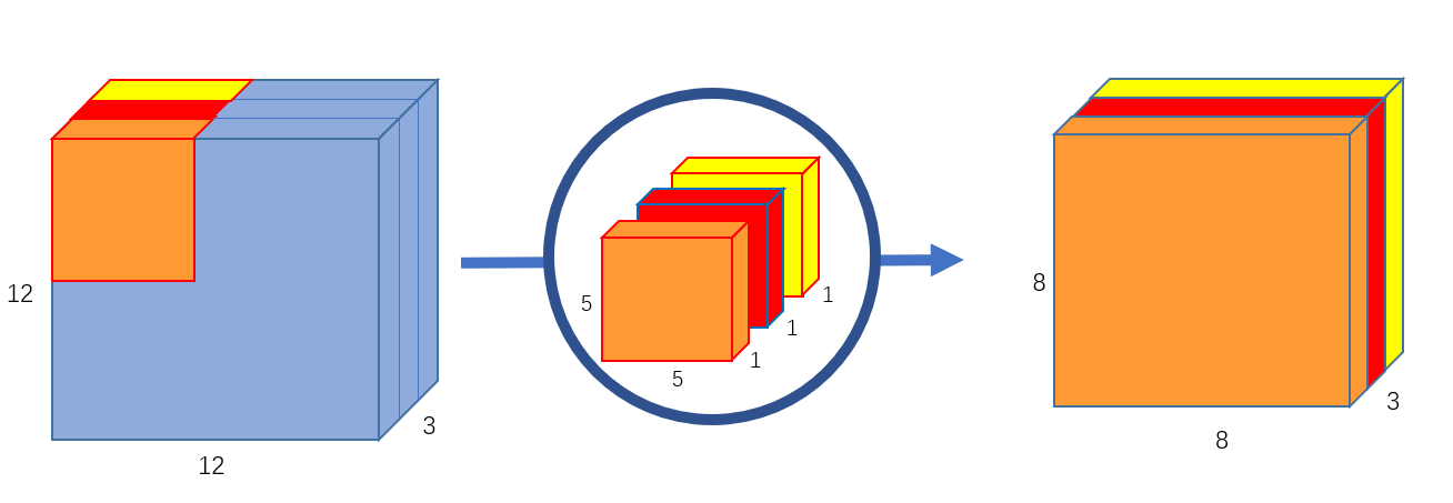
Depthwise Convolutions : While the normal convolution operation involves using filters that are as deep as the input tensor. For instance, if we’re doing a 2D Convolution on a $128 \times 128 \times 32$ tensor, we need our filters to have dimensions $k \times k \times 32$, where $k$ is the filter size. Obviously, having depth means having more parameters. Here comes the idea of Depthwise Convolutions, where instead of having deep filters, we have shallow filters operating on a slice of the depth of the input tensor. Thus, with Depthwise Convolutions, our filters each have a size of $k \times k$

2D Depthwise Convolutions using 3 filters of size 5x5. Figure source

Now considering the one-dimensional case: To output a matrix $O \in \mathbb{R}^{n \times d}$ using vanilla convolutions, we need $d$ filters each having size $d \times k$. This means that using normal convolutions, we need $d^{2} k$ parameters, while with depthwise convolutions, all we need are $d k$ parameters. See the figure below for a 1-dimensional depthwise-convolution on a $5 \times 5$ matrix with a filter of size $K=2$.

1D Depthwise Convolutions with a 2-sized filter

Lightweight Convolution: The proposed Lightweight Convolutions are built on top of three main components

1. Depthwise convolutions: explained above.
2. Softmax-normalization: That is, the filter weights are normalized along the temporal timension $k$ with a Softmax operation. This is a novel idea altough its partly borrowed from self-attention. Softmax Normalization forces the convolution filters to compute a weighted sum of sequence elements (words, tokens, etc.) and thus learn the contribution of each element to the final output.
3. Weight Sharing: To use even fewer parameters, the filter weights are tied across the embeddings dimension $d$ by grouping together every adjacent $d/H$ weights. This shrinks the parameters required even further from $dK$ to $HK$

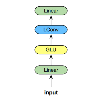
Lightweight Convolutions Module

As shown above, Lightweight Convolutions are preceded by a linear transformation mapping the input from dimension $d$ to $2d$, which is then followed by Gated Linear Unit (GLU). The GLU uses half of the input matrix as a gate by passing it to the sigmoid function, and then mutliplying elementwise by the second half. Then, another linear transformation is applied to obtain the output matrix $O$:

LConv Implementation : Upon reading the paper, I was very interested in knowing how lightweight convolutions were implemented. So, I took a look at the module implementation on Github. Interestingly, the authors implement LConv by transforming the convolution operation into matrix multiplication by a set of Band Matrices. Band Matrices are a type of sparse matrices where non-zero entries are concentrated around the main diagonal along with any other diagonals on either side. Below is an example of band matrix. They claim that this solution is faster than the existing CUDA convolutions on shorter sequences.

Example Band Matrix

Now let’s understand the implementation idea using an example. Given an input $X \in \mathbb{R}^{3 \times 4}$, imagine we’re about to do a lightweight convoution with a filter of size $K=2$, and using weight sharing where $H=2$ (meaning that $W \in \mathbb{R}^{H=2 \times K=2}$) and the input dimension $d=4$.

For instance let

Convolving $W$ around $X$ gives the following results:

Now let’s see how we can obtain this result using the band matrices methods. The preceding operation will be divided into $H=2$ different matrix multiplications of a band matrix with the relevant part of the input matrix. Which are the outputs of convolving using $W_{1,:}$ and $W_{2,:}$, respectively:

and

which are then combined to obtain the output matrix.

Now let’s take a look at the PyTorch implementation

The following lines expand and reshape the convolution filter weights in a way such that batch matrix multiplication can be done:

weight = self.weight.view(H, K)
weight = weight.view(1, H, K).expand(T*B, H, K).contiguous()
weight = weight.view(T, B*H, K).transpose(0, 1)

Now, we need to create the band matrices using the convolution filter weights. The as_strided function serves this purpose by creating a strided view into weight_expanded. It takes the output shape (B*H, T, K) and the strides or jumps we need to traverse the input array in each dimension which are :

• For the BH dimension we don’t need any strides so while traversing the array using that dimension, we need to jump total number of elements per one step T(T+K-1).
• For the temporal dimension T, we need a stride of one so we use we jump by the total number of elements T+K-1 our plus one element for the stride us T+K elements which are.
• for the last dimension, we have want no strides so we jump only one element at a time.

weight_expanded = weight.new_zeros(B*H, T, T+K-1, requires_grad=False)
weight_expanded.as_strided((B*H, T, K), (T*(T+K-1), T+K, 1)).copy_(weight)# creating the band matrices using the
# as_strided function
weight_expanded = weight_expanded.narrow(2, P, T)

Ok, How about Dynamic Convolutions?

One limitation of Lightweight Convolutions as opposed to self-attention is that the weights assigned to sequence elements do not change according to context. That is, the convolution weights used at the timestep $i$ are the same when sliding the filter one more step at $i+1$.

Dynamic Convolutions remedy that by using a time-dependent kernel that changes dynamically based on the current timestep (Not the whole context as with self-attention):

where $f(X_i)$ is a matrix computed by means of a linear transformation with learnt weight matrix $W^Q \in \mathbb{R}^{H \times k \times d}$. Thus, the filter weight for positions for position $j$ and head $h$ are computed by \(\sum_{c=1}^{d}W_{h,j,c}^{Q}. X_{i,c}\).

Note that to compute the attention weights, the above equation will be computed at $O(n)$ times in contrast to computing self-attention which computed them in $O(n^2)$ (The cost of multiplying $KQ^{T}$. Dynamic Convolutions are very memory hungry (just look at $W^Q$!). So, it was essential to shrink the number parameters through both Depthwise operation and weight sharing, in order to be able to implement Dynamic Convolutions on current hardware.

Conclusion

In this article, we saw how the simple but interesting idea of Lightweight Convolutions originated. We also discussed how it is partly based on Depthwise Convolutions, Softmax normalization and weight sharing. We delved into the implementation idea and source code used by the authors where convolution was implemented as a batch matrix multiplication by a set of band matrices. Finally, we explored the interesting concept of time-depended kernels where convolution weights are not fixed but rather depend on the current timestep.