Paper Discussion: Discrete Generative Models for Sentence Compression
I will discuss the 2016 paper Language as a Latent Variable: Discrete Generative Models for Sentence Compression. The reason why I chose this paper is two-fold : First, it combines a lot of important ideas and concepts such as Variational Auto Encoders, Semi-Supervised learning and Reinforcement Learning.
Haven’t posted in a while, but I decided to get back and get back strong! In this post, I will discuss the 2016 paper Language as a Latent Variable: Discrete Generative Models for Sentence Compression. The reason why I chose this paper is two-fold : First, it combines a lot of important ideas and concepts such as Variational Auto Encoders, Semi-Supervised learning and Reinforcement Learning. Second, it’s relevant to my master’s thesis and I find that writing about a topic help make it clearer.
Paper Brief
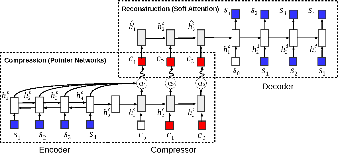
The main idea of the paper is that an autoencoder that takes a sentence as input, should learn to map that input into a space where important information regarding the sentence are kept, such that the model is able to reconstruct the sentence again. By enforcing this intermediate representation (Latent Variable) to be in the form of a discrete language model distribution (a valid sentence), we are able to learn a compact version of the input sentence.
Variational Autoencoders
Variational Autoencoders are typical autoencoders with the exception that the latent variable distribution should exhibit a gaussian prior. This pushes the encoder to output diverse and geometrically regular representations. It also prevents the encoder from cheating by assigining each image a distinct point in space. The loss function of the VAE is split into two parts: Decoder Loss and KL Divergence between the encoder posterior and the prior of the latent variable $z$:
\[\begin{equation} L(\theta, \phi) = -\mathbb{E}_{z \sim q_{\phi}}[log p_{\theta}(x|z)] + KL (q_{\phi}(z|x) || p(z)) \end{equation}\]| Where $\theta$ are the decoder parameters and $\phi$ are the encoder parameters. Note that this loss is the negative of what is known as the variational lower bound of the model. It can be proven that maximizing the lowerbound is equivalent to minimizing the KL Divergence between the true posterior $p(z | x)$ and the approximate posterior $q(z | x)$. Check out this amazing post to understand more. In the paper we discuss, the compressed form of the sentence is treated as the latent variable (hence the name of the paper), which is then used to reconstruct the original sentence again. |
Compression model
Back to our language generation setting, the encoder is a bi-LSTM encoding the input sentence. Following that, another pointer network attends over the encoder states to produce the compressed input sentence. These two networks form the compression model $q_{\phi}(c|s)$
Reconstruction model
This includes the compressor and the decoder together outputting the reconstructed sentence with probability $p_{\theta}(s|c)$. The reconstruction occurs as follows: the compressor LSTM encodes the compressed sample. Then, the decoder LSTM attends to the compressor hidden states to output the reconstructed sentence
Unsupervised Model Training
- Reconstruction model : Decoder parameters $\theta$ are updated directly with gradient ascent.
We’re using gradient ascent to since we want to maximize the variational lower bound \(\begin{equation} L = \mathbb{E}_{c \sim q_{\phi}(c|s)}[log p_{\theta}(s|c)] - KL (q_{\phi}(c|s) || p(c)) \end{equation}\)
Also note that the compressor parameters are not updated by the gradients from the reconstruction model
- Compression model : The non-differentiability of the compression model imposes using a different training strategy. The authors employed the REINFORCE algorithm which is a standard policy training algorithm for Reinforcement Learning problems.
First, a learning signal (similar to rewards in policy gradients) is defined as :
\[l(s,c) = log p_{\theta}(s|c) - \lambda (log q_{\phi}(c|s) - log p(c))\]where $\lambda$ is a hyperparameter used to control the weight of the KL divergence on the objective function. During experiments, $\lambda$ was set to 0.1 to reduce the effect of the compression since the pretrained-language model$p(c)$ tends to prefer shorter sentences. If compressed sentences are very short, this will force the decoder to rely on its own outputs rather than the output from the compressor.
Then the compression model parameters are updated with:
\[\begin{equation} \frac{\partial L}{\partial \phi} = \mathbb{E}_{q_{\phi(c|s)}} [l(s,c) \frac{\partial log q_{\phi}(c|s)}{\partial \phi}] \end{equation}\]This can be intuitively explained as trying to maximize the probability of outputting compressed sentences for which the learning signal is positive and minimizing it for those with negative learning signals. This is very similar to policy gradients where you are encouraging actions with positive reward and discouraging ones with negative reward. They also introduce an input-dependent baseline (Simple MLP) to reduce the variance of the gradients.
Supervised Model Training
In addition to the Autoencoder Sentence Compression (ASC) model, another model is introduced, that is the Forced Attention Compression model (FCS) to train the model. At each step, the FSC model chooses to either copy a word from the input (as in a traditional pointer network) or generate a new word from the vocbulary. This model is typically trained in a supervised fashion buy exploiting parallel sentence-compressed pairs.
Semi-Supervised Training
Exploiting both unlabeled $\mathbb{U}$ and labeled parallel data $\mathbb{L}$, the authors introduced a mixed objective function \(\begin{equation} J = \sum_{s \in \mathbb{U}} \mathbb{E}_{c \sim q_{\phi}(c|s)}[log p_{\theta}(s|c)] - KL (q_{\phi}(c|s) || p(c)) + \sum_{s \in \mathbb{L}} p_{\phi}(s|c) \end{equation}\)
Combining a reinforcement learning loss with a cross entropy loss has been used extensively recently due to that using cross-entropy only suffers from Exposure Bias which is the discrepancy between the training and testing procesures, that is, the model is trained using the forced outputs from the dataset but is tested using its own generated outputs.