Step-by-Step Text Classification Tutorial using Tensorflow
In this post, I will walk you through using Tensorflow to classify news articles. Before you begin, you should have tensorflow, numpy and scikit-learn installed.
import tensorflow as tf
import numpy as np
from sklearn.datasets import fetch_20newsgroups
from sklearn.feature_extraction.text import TfidfVectorizer
from sklearn import metrics
Importing twenty-newsgroup dataset
the twenty-newsgorup datasets is a collection of news articles.
Each article is labeled according to its type for example : medical news, automobile news,…etc.
In this tutorial we will deal with 4 classes of articles.
categories = ['rec.autos', 'comp.graphics', 'sci.med', 'sci.electronics']
no_classes = len(categories)
twenty_train = fetch_20newsgroups(subset='train',
                                  categories=categories,
                                  shuffle=True)
twenty_test = fetch_20newsgroups(subset='test',categories=categories,shuffle=True)
TF-IDF statistic
We will use the bag-of-words model to represent each article.
There are a couple of variations of that model: term frequency , which represents each document as a vector of word counts, also there is term frequency-inverse document frequency which is the same as tf except that each word is weighted by its significance to that article.
Luckily for us, scikit-learn has a class just for that.
tfidf = TfidfVectorizer()
train_x = tfidf.fit_transform(twenty_train.data)# fit on training data
train_y = twenty_train.target # train target values
test_x = tfidf.transform(twenty_test.data) # transform test data to tfidf representation
test_y = twenty_test.target
Preparing data for training
When doing classification using neural networks, we must have an output layer with k neurons where k is the total number of classes. If an instance belongs to a certain class, the output value for the corresponding neuron for that class should be 1 and all other values should be zero. Thus to be able to train our neural network, we have to transform the class labels of the articles to a vector having 1 at the correspoing label and 0 at all other positions. This type of vectors is known as one-hot vector.
# transforming target classes into one-hot vectors
def vector_to_one_hot(vector,no_classes):
    vector=vector.astype(np.int32)
    m = np.zeros((vector.shape[0], no_classes))
    m[np.arange(vector.shape[0]), vector]=1
    return m

train_y =vector_to_one_hot(train_y,no_classes)
test_y = vector_to_one_hot(test_y, no_classes)
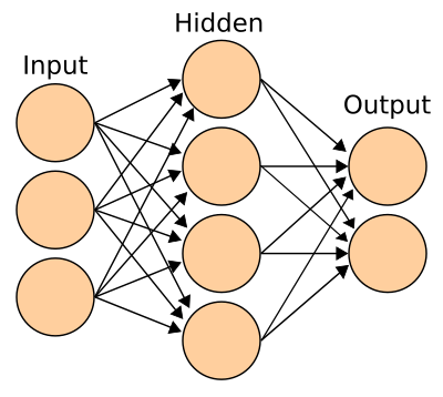
We’ll use a very simple architecture like the one shown in the picture. However, we’ll an input layer of size equal to the vocabulary size, A hidden layer of our choice and an output layer of 4 output neurons corresponding to the 4 classes we have.
Setting model parameters
# Parameters
learning_rate = 0.1
num_steps = 500
batch_size = 16
display_step = 100

beta = 1 # regularization parameter
# Network Parameters
n_hidden_1 = 8 # size of 1st hidden layer

num_input = train_x.shape[1] #input vector size
num_classes = no_classes
Defining input and output
With tensorflow, inputs and outputs to network are defined as placeholders.
The training data is the fed to these placeholder at training time.
Note we define the first dimension to be None meaning we don’t have a fixed input size (batch size) and tensorflow will deduce that at training time.
X = tf.placeholder("float", [None, num_input]) # place holder for nn input
Y = tf.placeholder("float", [None, num_classes]) # place holder for nn output
Defining weights
Since our network has only one layer (you can add layer if you want), we will have two sets of weights : From input layer to the hidden layer and from the hidden layer to the output layer.
weights = {
    'h1' : tf.Variable(tf.random_normal([num_input, n_hidden_1])),
    'out': tf.Variable(tf.random_normal([n_hidden_1,num_classes]))
}

biases = {
    'b1': tf.Variable(tf.random_normal([n_hidden_1])),
    'out': tf.Variable(tf.random_normal([num_classes]))
}
Tie everything together
def neural_net (X):
    layer_1 = tf.add(tf.matmul(X, weights['h1']),biases['b1'])
    layer_1 = tf.nn.sigmoid(layer_1)
    out_layer = tf.add(tf.matmul(layer_1,weights['out']), biases['out'])
    out_layer = tf.nn.sigmoid(out_layer)
    return out_layer
We define our loss function to be cross entropy with softmax probabilities. Tensorflow has a function to compute that.
The idea of using cross entropy is to maximize the probability of the correct class. So by minimizing the loss (negative log probability), we are maximizing the probabilty of the correct label.
Optimization is done by means of the ADAM optimization method which is somehow more efficient than SGD.
logits = neural_net(X)
loss = tf.reduce_mean(
    tf.nn.softmax_cross_entropy_with_logits(logits=logits,labels=Y))

loss = tf.reduce_mean(loss)
optimizer = tf.train.AdamOptimizer(learning_rate)

train_step = optimizer.minimize(loss)

#evaluate model
correct_pred = tf.equal(tf.argmax(logits,1), tf.argmax(Y,1))
accuracy = tf.reduce_mean(tf.cast(correct_pred, tf.float32))
y_pred = tf.argmax(logits,1)
init = tf.global_variables_initializer()
To get less training time, we divide training data into batches and perform all weights updates for all instances in the batch at one.
This method returns the next batch of given training data with the specified batch size
def get_train_batch(batch_size,train_x,train_y):
    global train_index

    if train_index + batch_size >= train_x.shape[0]:
        train_index += batch_size
        return train_x[train_index:,:],train_y[train_index:,:]# false to indicate no more training batches
    else :
        r= train_x[train_index:train_index+batch_size,:],train_y[train_index:train_index+batch_size,:]
        train_index += batch_size
        return r
with tf.Session() as sess:
    sess.run(init)
    train_index=0
    moreTrain = True
    step = 0
    while True:
        step+=1
        if train_index >= train_x.shape[0] : break
        batch_x , batch_y = get_train_batch(batch_size,train_x.todense(),train_y)
        sess.run(train_step, feed_dict={X:batch_x,Y:batch_y})

        if step % 10 == 0 :

            cur_loss,cur_accuracy = sess.run([loss,accuracy],feed_dict={X:batch_x,Y:batch_y})
            print ('loss = %.2f , accuracy = %.2f , at step %d' %(cur_loss, cur_accuracy,step))


    print ("done optimization")
    y_p = sess.run(y_pred,feed_dict={X:test_x.todense(),
                                      Y:test_y})
    print("Testing Accuracy:", \
        sess.run(accuracy, feed_dict={X: test_x.todense(),
                                      Y: test_y}))
    print ("f1 score : ",
          metrics.f1_score(twenty_test.target, y_p,average='macro'))
loss = 1.30 , accuracy = 0.38 , at step 10
loss = 1.18 , accuracy = 0.88 , at step 20
loss = 1.02 , accuracy = 0.75 , at step 30
loss = 0.97 , accuracy = 0.88 , at step 40
loss = 0.90 , accuracy = 0.88 , at step 50
loss = 0.84 , accuracy = 0.94 , at step 60
loss = 0.86 , accuracy = 0.88 , at step 70
loss = 0.77 , accuracy = 1.00 , at step 80
loss = 0.83 , accuracy = 0.94 , at step 90
loss = 0.80 , accuracy = 1.00 , at step 100
loss = 0.75 , accuracy = 1.00 , at step 110
loss = 0.76 , accuracy = 1.00 , at step 120
loss = 0.78 , accuracy = 0.94 , at step 130
loss = 0.84 , accuracy = 0.88 , at step 140
done optimization
Testing Accuracy: 0.914867
f1 score :  0.914819748906
We can see we have a very good accuracy and f1-score on test data.
Comparing to SVM
from sklearn.svm import SVC
clf = SVC(kernel='linear')
clf.fit(train_x,twenty_train.target)
SVM Testing accuracy :  0.91041931385
SVM F1-score :  0.910699838044
we can see the NN approach slightly outperforms the SVM. I strongly suggest You try on your own to play a little with the neural network layer structure and hyperparatmers and try to further improve its performance. You can also add regularization and see how it goes.
Conclusion
In this tutorial we applied a simple neural network model on text classification. We represented our articles using TF-IDF vector space represenation. We then used cross entropy as our loss function. We trained the model and got very good accuracy and f1-score. We also tried and SVM model on the data and compared perfomance between the two models.